On this page I will provide some general guidance on how to use the TI-83 & TI-84 84 calculators’ most important functionalities.

Note for SAT and AP exams

If you are taking a CollegeBoard exam (PSAT, SAT, AP, etc.), all assessments are now digital and now include access to the Desmos graphing and scientific calculators. The Desmos calculators are much faster and more powerful than TI calculators and are recommended to use for these exams instead of the TI calculators for students that are familiar with them. Familiarity with TI calculators can still be helpful for traditional school exams, though, so there skills are not totally obsolete (yet).

This page is a continual work in progress and more features will be added as time goes on.

Graphing Functions

Inputting Functions to Graph

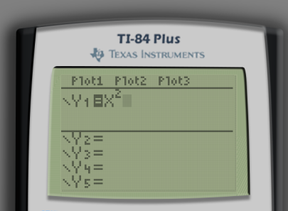
To graph a function, say $y = x^{2}$ , click the Y= button and type in your function on the Y₁= line. In order to type in X, use the X,T,θ,n button or ALPHA followed by STO→.

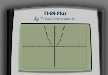
Then, click the GRAPH button to show the graph of the function. By default each tick mark on the screen represents $1$ unit in each direction.

Displaying Your Graph Properly

By default the graph will show $x$ values from $- 10$ to $10$ and $y$ values from $- 10$ to $10$ . More compactly, we can write this window setting as $[- 10, 10] \times [- 10, 10]$ (the first interval indicates the $x$ values and the second interval indicates the $y$ values). Since by default these $x$ and $y$ values run to the same values in each direction ( $\pm 10$ ) and the calculator’s screen is a rectangle, the graph gridlines are actually squished in the vertical direction.

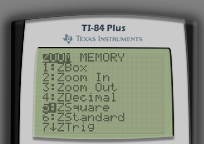
If you want to the display so that the proportions are correct, go to ZOOM and select the 5:ZSquare option.

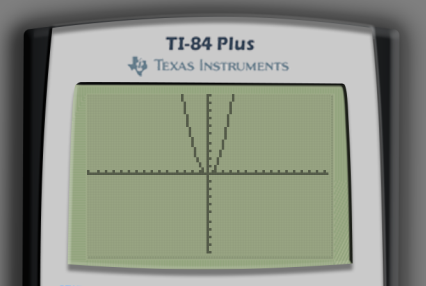
Here is the graph view with fixed proportions.

The impact is more obvious when comparing the graph of a circle before and after using 5:ZBox. (I used the equations $y = 25 - x^{2}$ and $y = - 25 - x^{2}$ , which together form the circle of radius $5$ centered at the origin.)

Before using `5:ZBox`	After using `5:ZBox`

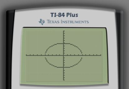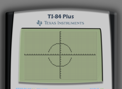Ignore the fact that the circle does not appear entirely connected. This is just an artifact of how the calculator does the computations to create its graphs. Calculators like Desmos fix this issue as they have much higher computational resolution.

To return back to the default zoom, click ZOOM and select 6:ZStandard.

The `WINDOW` Menu

Click WINDOW to see the current settings pertaining to which part of the graph gets shown on the screen and modify these values directly.

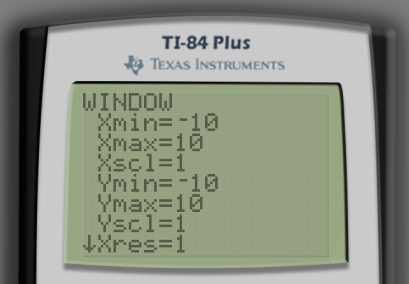
Each of the values shown here can be modified based on your particular preferences. Here is what each of them mean.

Property	Interpretation
`Xmin`	$x$ value for the left-hand edge of the window
`Xmax`	$x$ value for the right-hand edge of the window
`Xscl`	the number of units each $x$ axis tick mark represents
`Ymin`	$y$ value for the lower edge of the window
`Ymax`	$y$ value for the upper edge of the window
`Yscl`	the number of units each $y$ axis tick mark represents
`Xres`	horizontal distance between plotted points in pixels*
`Δx`	the width of each pixel measured in $x$ units**

*This value accepts only whole number values $1$ – $5$ . Higher values of Xresmake for a faster graphing experience but the resulting images will appear increasingly jagged.

**Changing Δx will cause the Xmax value to update to match and vice versa.

The `ZOOM` Menu

Click ZOOM to access options that allow you to zoom in and out of the graph.

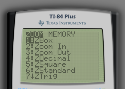
This menu is enormous so I will only describe the most important zoom features below. I use all of these five features outlined below with regularity and I strongly recommend practicing using these Zoom features on a graphed function.

Option	Functionality
`1:ZBox`	Marquee zoom: After selecting this option, a tool will be opened that lets you select a rectangular portion of the existing graph to zoom in on. Use the arrow keys and the `ENTER` button to make the rectangular selection and then zoom.
`2:Zoom In`	Zoom into your graph centered around the cursor. After selecting this option, move the cursor with the arrow keys and press `ENTER` to zoom. Proportions are preserved.
`3:Zoom Out`	Zoom out from your graph centered around the cursor. After selecting this option, move the cursor with the arrow keys and press `ENTER` to zoom. Proportions are preserved.
`5:ZSquare`	Adjusts `Ymin` and `Ymax` so that the graph is displayed with proper proportions.
`6:ZStandard`	Reset the graphing window to default $[- 10, 10] \times [- 10, 10]$ . Warning: This does not provide proper proportions.

Solving Any Equation (Approximately)

Let’s say we have a complicated equation that cannot be solved by hand.

\frac{1}{x + 3} = 3 x + 2^{x}

First, in Y= type in the left-hand side and right-hand side into the first two lines.¹ It doesn’t matter which comes first.

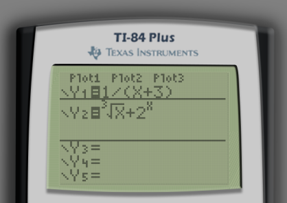
Graph the two functions and make sure their intersection(s) are visible on the screen. For this example, the 6:ZStandard window $[- 10, 10] \times [- 10, 10]$ suffices.

If you desire finer detail, though, I recommend doing a 1:ZBox to show both intersections at a higher zoom level.

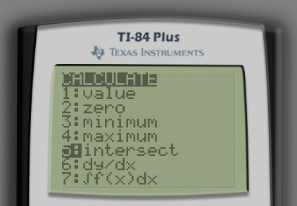
We can see that our equations intersect twice. This means that we have two solutions. The $x$ coordinates of the two intersection points are the two solutions to our original equation. In order to find the intersection points, press the 2ND button followed by the TRACE button in order to open the CALC menu. Then, select 5:intersect.

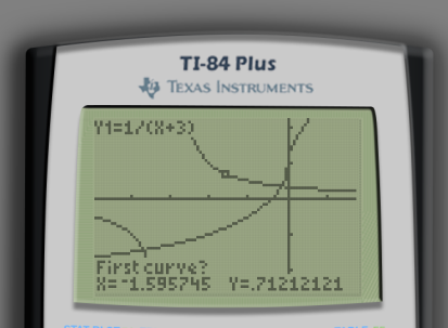
The calculator will ask First curve?. More likely than not, one of the equations that you are working with will be displayed at the top of the screen. In my case, the calculator displays Y1=1/(X+3) at the top-left of the screen. This is one of the equations that we are working with for our intersection so just press ENTER. If the correct equation isn’t indicated by default, press the ↑ and ↓ keys until the correct equation is displayed.

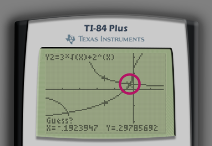
After pressing ENTER, the calculator will ask Second curve?. Ensure that the function corresponding to the other side of the original equation is displayed at the top-left of the screen using the same process and press ENTER. Indeed, Y2=3ˣ√(x)+2^(x) is the function for the other side of our equation.²

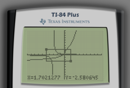
After pressing ENTER, the calculator will ask Guess?. Move the cursor with the arrow keys to the location of one of the intersections. For clarity, I have circled the location of my cursor in the following screenshot.

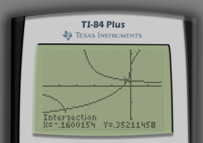
After pressing ENTER, the calculator will estimate the coordinates of the intersection point, usually to reasonable accuracy.

Repeat this process for the intersection point at the bottom-left of the screen.

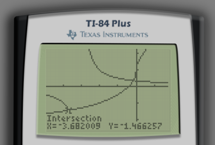
Reading off the $x$ coordinates of the intersection points, the approximate solutions to our equation are as follows.

x \approx {- 0.1600154, - 3.862009}

Finding the Maximum/Minimum Value of a Function

Information coming soon!

In order to input a cube root, click MATH and select 4:³√(. ↩
In the language of the calculator, 3ˣ√(x) is the same as ³√(x) which represents $3 x$ . (This is an archaic notation that was carried through for purposes of displaying the necessary information when pixel space is limited.) ↩

Trevor's Notes

Explorer

TI Calculator Reference

Table of Contents

Graphing Functions

Inputting Functions to Graph